National Marine Sanctuary of American Samoa

Ocean Sound Monitoring

The National Marine Sanctuary of American Samoa (NMSAS) is comprised of six protected areas, covering 13,581 square miles of nearshore coral reef and offshore open ocean waters across the Samoan Archipelago. The sanctuary protects extensive coral reefs, including some of the oldest and largest Porites coral heads in the world, along with deep-water reefs, hydrothermal vent communities, and rare marine archaeological resources.

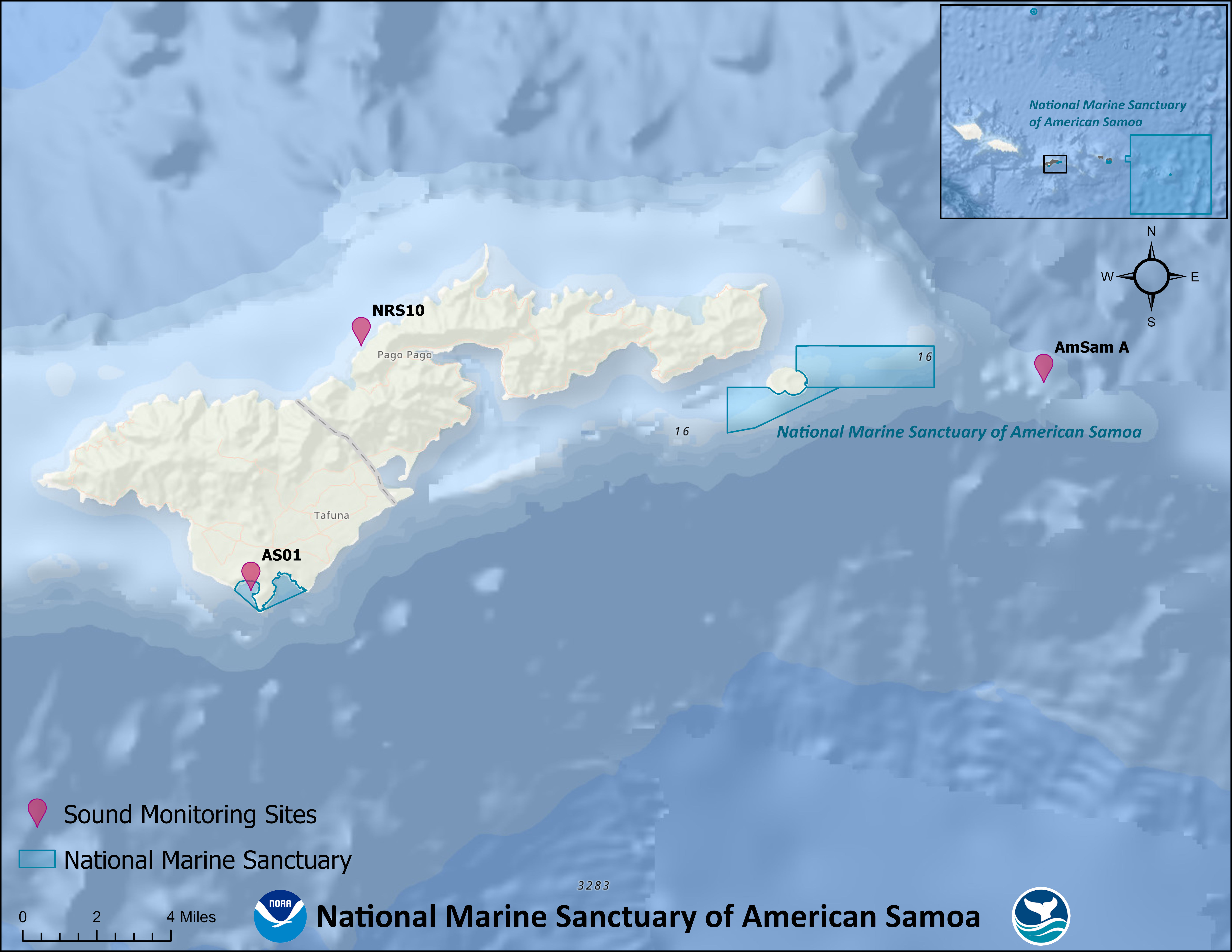
Ocean sound monitoring coordinated by ONMS began in 2023 through the ONMS Sound program, building on historical efforts to characterize the underwater soundscape around American Samoa. Current monitoring and analysis are conducted at one site (AS01) within NMSAS. In addition, two monitoring sites located outside of sanctuary boundaries provide broader context: the Noise Reference Station (NRS 10), established in 2015, and a NOAA Fisheries deep-water site (AmSam) deployed in 2023. Together, these sites support long-term monitoring of soundscape conditions both inside and outside the sanctuary to help inform sanctuary management.

Summary of monitoring sites

Long-term Monitoring Site	Primary Monitoring Purpose	Oceanographic Setting	Depth (m)	Sampling Rate (kHz)	Known Biological Sounds	Vessel Traffic Setting	Latitude	Longitude	StartDate	Total Recording Days
AS01	A shallow reef site within Fagatele Bay selected for exceptional biodiversity, likely among the highest in the National Marine Sanctuary System, supporting diverse coral, invertebrates, fishes, marine mammals, and turtles. Established to monitor reef health, human use, and marine mammal presence.	coastal-shallow	22	48	Humpbacks (Aug-Oct), fish, odontocetes, and snapping shrimp	No-take zone	-14.28	-170.45	March 2023	72
NRS10	Part of Ocean Noise Reference Station (NRS) network, established to monitor long-term trends in ocean noise, baleen whale species presence, and vessel noise.The site is Tutuila Island, and management is shared with the U.S. National Park Service.	coastal-shallow	33	5	Humpbacks (Aug-Oct) and fish	Minimal traffic	-14.27	-170.72	June 2015	1048
AmSam	A deep-water site managed by NOAA Pacific Islands Fisheries Science Center. The site was established to monitor marine mammal presence and anthropogenic activity.	offshore-deep	750	200	Humpbacks (Aug-Oct), baleen whale species, and odontocetes	Minimal traffic	-14.28	-170.45	July 2023	290

Ocean Sound Conditions

Soundscapes vary across years, seasons, and even within a day. Differences are driven by shifts in wind and weather patterns, migration and behavior of animals, and patterns in human activities. We track how sound levels change in different frequencies using standardized soundscape metrics to understand these changes. Seasonal and annual percentiles of all the data, a measurement of data spread with the middle 50% falling between the 25th and 75th percentile, are used to define typical conditions.

What are the seasonal patterns across frequencies?

Season is often a main driver of soundscape differences: wind and weather patterns shift, species migrate or change behavior, and humans change their marine activities. As shown on the graphic(s) below, we can visualize the differences by looking at the variation across frequency (pitch of the sound in Hertz) shown on the x-axis and intensity (how loud the sound is in decibels) shown on the y-axis. The colored lines represent regionally-specific oceanographic seasons, vertical shaded bars are the frequency ranges that a sound source of interest can be heard, and the black lines bound the expected range of modeled sound intensity when only wind noise is present.
Here are some questions to consider when viewing the graph(s) below:
(1) Which season has the highest sound levels?
(2) Are there peaks in the sound levels for any of the sounds of interest?
(3) Are the low-frequency sound levels outside the expected range for wind noise?

Seasonal median sound levels (sound intensity measured by mean-square pressure in microPascal per Hertz) across a range of frequencies (~10 to ~24,000 hertz) at a given monitoring site, with annual recording effort represented by a bar graph underneath. Each season is a different colored line. Solid black lines show modeled ambient sound levels from wind at 1 m/s (lower line) and 22.6 m/s (upper line) based on hydrophone depth. Frequency bands indicative of a biological or anthropogenic sound source of interest are highlighted in semi-transparent gray and labeled; peak frequency for dominant fish species are labeled with vertical dashed lines. Credit: Megan McKenna and Emma Beretta/CIRES and NOAA

Processing raw audio files to calibrated sound levels (i.e., soundscape metrics) involves multiple steps to get a specified time frequency data product. All soundscape metrics visualized in the soundscape inventory reports are averaged from hybrid millidecade sound levels, calculated using either MANTA or PyPAM software packages. Both softwares calculate mean PSD (dB re 1 µPa^2/Hz) per minute in 1-Hz wide bins using Welch’s method with a Hann window, FFT length equal to the sample rate, and 50% overlap. Following calibration based upon instrument specific sensitivities, PSD values per minute were further processed in hybrid millidecade spectral densities, which are an efficient means of storing PSD spectra from high sample rate audio files using 1-Hz values up to 435 Hz, and then millidecade wide PSD values up to one half of the sample rate (Martin et al. 2021).

PAMscapes was used to calculate hourly median hybrid milli-decade bands (loadSoundscapeData(ncFile, keepQuals = c(1,2)) and binSoundscapeData(hmddata, bin = "1hour", method = c("median")). The hourly data were then matched with an estimate of wind speed at that location using matchGFS in PAMscapes (Global Forecast System (GFS) weather model). Long-term condition plots in these reports were generated by averaging the hourly median hybrid millidecade results within different time constraints (i.e. annual, seasonal) and percentiles (e.g., 25% and 75%) for each hybrid millidecade frequency band.

How are ocean sound conditions changing across years?

We can track changes in ocean soundscape conditions and its contributors by comparing annual sound levels. Efforts to reduce noise impacts to marine animals are underway on local to global scales. Strategies can include avoidance of times and areas when sensitive species are present to reduce vulnerability (e.g., a shipping lane), changing the operation of a potentially hazardous noise source (e.g., by slowing and therefore quieting vessels) or through the design and use of alternative, quieter sources (e.g., new, quieter ship design and/or technologies). The effectiveness of these approaches, and the scales over which they are effective, can be tracked through comprehensive monitoring efforts. A focused analysis is often necessary to tease apart the multiple drivers of ocean sound levels, however, annual summaries provide initial insights to overall patterns.
Here are some questions to consider when viewing the graph(s) below:
(1) Are levels lower in the most recent year of monitoring in any of the frequencies of interest?
(2) Are there peaks in the sound levels for any of the sounds of interest? Do they differ across years?

Annual median sound levels (sound intensity measured by mean-square pressure in microPascal per Hertz) across a range of frequencies (~10 to ~24,000 hertz) at a given monitoring site, with annual recording effort represented by a bar graph underneath. Each year is a different blue line, getting darker for every additional year of data. Solid black lines show modeled ambient sound levels from wind at 1 m/s (lower line) and 22.6 m/s (upper line) based on hydrophone depth. Frequency bands indicative of a biological or anthropogenic sound source of interest are highlighted in semi-transparent gray and labeled; peak frequency for dominant fish species are labeled with vertical dashed lines. Credit: Megan McKenna and Emma Beretta/CIRES and NOAA

Is the intensity (loudness) of sound sources of interest within typical range?

In some soundscapes, we can use specific frequencies as indicators for the presence of a source of interest (e.g. species presence and behavior). Monitoring sites are often chosen because a known source that we want to track is present and we can track this dominant sound energy contributor using their specific frequency or frequency range. For example, seasonal migration of humpback whales to Hawaiian Islands results in soundscapes dominated by their calling between 50 and 630 Hz. At sites near commercial shipping lanes, 63 and 125 Hz one-third octave level (TOL) are used as an indicator for ship noise (Haver et al. 2021)). At sites where snapping shrimp are present, 4,000 - 18,000 Hz can be used as an indicator of their sounds. Only frequencies that have been identified as reliable for tracking a source of interest are shown below.

Time series plot of daily median sound levels (sound intensity measured by mean-square pressure in microPascal per Hertz) for a specific frequency band(s) of interest at this site, separated by year. Background color shading (blue, purple, gold) indicates low (<25th percentile), typical (25-75th percentile), and high sound levels (>75th percentile) across this monitoring site's entire dataset at this frequency band(s) for comparability with annual medians, marked with horizontal black dashed lines. Pie charts on the right hand side of the graphic show the proportion of daily median sound levels that fell within each category for each year, following the same color-coding and percentile bins. Credit: Megan McKenna and Emma Beretta/CIRES and NOAA

Ocean Sound Indicators

We can use long-term monitoring of ocean sound to derive and track indicators of ocean conditions. These indicators track the status and trend of habitat condition, species presence, human-use patterns, and management activities. There are many analytical methods used to generate ocean sound indicators. Below are ocean sound indicators relevant to the sanctuary and available for condition tracking.

When do fish contribute to the soundscape?

ONMS partnered with Conservation Metrics to analyze acoustic data collected across Pacific Island Region sites. Conservation Metrics developed a machine learning classification model to process these large datasets, enabling the detection and classification of acoustic signals. Patterns in fish activity, including both sound production and behaviors like grazing, help identify key biological periods and offer insight into the health and function of coral reef ecosystems. The model grouped fish sounds into seven aggregate classes. Here we focus on one of these classes: damselfish.

The heatmap of damselfish detections shows activity per minute for each hour and day of the dataset. Date is on the x-axis, time of day is on the y-axis, and color represents detections per minute.

Heatmap showing mean detections per minute of damselfish at site AS01 (Fagatele Bay) in National Marine Sanctuary of American Samoa from late March to end of May 2023. Time of day is on the y-axis (0:00–24:00) and date on the x-axis. Color intensity represents detection rate, with darker colors indicating fewer detections and lighter colors indicating higher detections. The gray solid and dashed lines mark times of dawn and dusk. Credit: Conservation Metrics