Hawaiian Islands Humpback Whale National Marine Sanctuary Soundscape Report

Ocean Sound Monitoring

Every winter, thousands of humpback whales travel to the warm, shallow waters of Hawai‘i to mate, give birth, and raise their young. Hawaiian Islands Humpback Whale National Marine Sanctuary (HIHWNMS) protects these whales and their habitat.

Ocean sound monitoring coordinated by ONMS began in 2018 through the Sanctuary Soundscape Monitoring Project. However, a long history of underwater acoustic monitoring has occurred in this sanctuary from various partners and organizations.

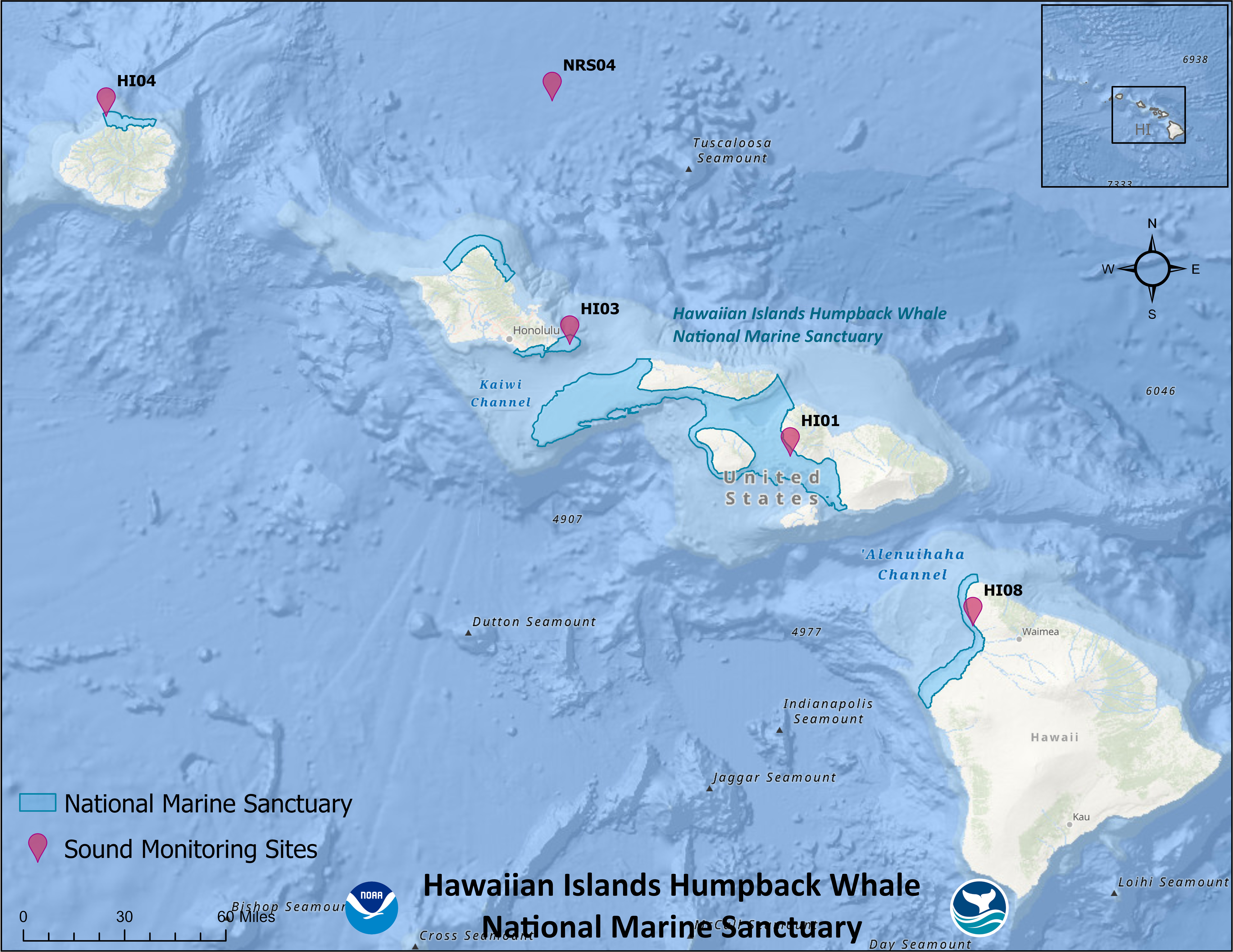
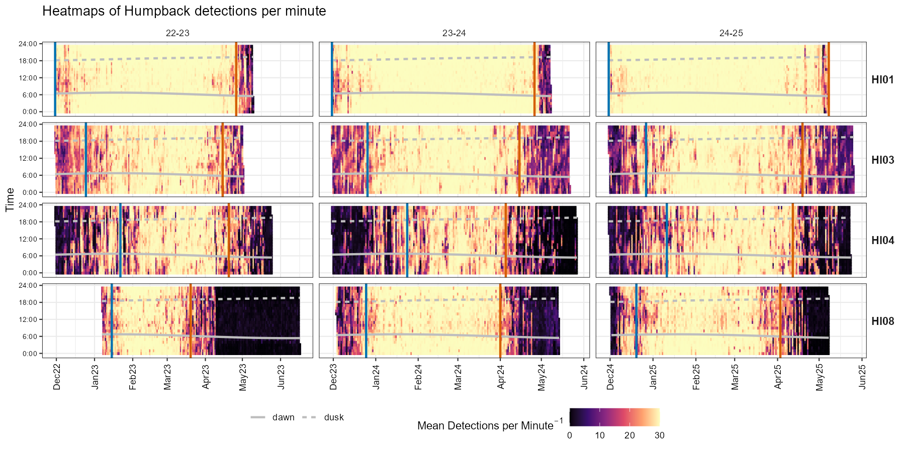
Current ONMS ocean sound monitoring and analysis is maintained at four sites within HIHWNMS. These sites (HI01, HI03, HI04, HI08) continue to support monitoring of humpback whale migration and habitat use patterns as well as vessel traffic from commercial activities, including whale watching. In addition, one monitoring site outside sanctuary boundaries, the Noise Reference Station (NRS 04), established in 2015, provides a baseline for ocean sound conditions beyond the sanctuary.

To see historical monitoring sites that are no longer active, please visit Sanctuary Soundscape Project data portal.

Summary of monitoring sites

Long-term Monitoring Site	Primary Monitoring Purpose	Oceanographic Setting	Depth (m)	Sampling Rate (kHz)	Known Biological Sounds	Vessel Traffic Setting	Latitude	Longitude	StartDate	Total Recording Days
HI01	Area located off west Maui with high humpback whale densities and vessel activity adjacent to Olowalu Reef. Monitoring focuses on long-term trends in humpback whale migration and habitat use. Acoustic monitoring at this site has revealed that the timing and abundance of whales off west Maui has fluctuated in recent years.	coastal-shallow	62	48	Humpbacks (Dec-May), fish, odontocetes, and snapping shrimp	Commercial and recreational vessel noise	20.81	-156.66	Dec 2018	739
HI03	Large bank off of southeast Oahu with relatively high humpback whale densities and anthropogenic activity, providing a key comparison to other sites and continuing long-term monitoring of whale migration and habitat use.	coastal-shallow	79	48	Humpbacks (Dec-May), minke whales (Oct-May), fish, and odontocetes	Commercial and recreational vessel noise	21.29	-157.6	Dec 2022	503
HI04	A site off the north shore of Kauai with relatively high humpback whale densities adjacent to the Navy’s Pacific Missile Range Facility, where naval training exercises occur. Monitoring focuses on long-term trends in humpback whale migration and habitat use, as well as anthropogenic activity.	coastal-shallow	80	48	Humpbacks (Dec-May), minke whales (Oct-May), fin whales, fish, and odontocetes	Commercial, military and limited recreational vessel noise	22.26	-159.59	Dec 2022	352
HI08	An area off the northwest coast of Hawai‘i Island with relatively high humpback whale densities near the historical SanctSound site HI06. Exposed to deeper offshore waters and located ~7 km from Kawaihae Harbor, the site captures a range of marine mammals and vessel traffic. Monitoring at this site focuses on long-term trends in humpback whale migration and habitat use, as well as anthropogenic activity.	coastal-shallow	64	48	Humpbacks (Dec-May), fish, odontocetes, and snapping shrimp	Commercial and recreational vessel noise	20.09	-155.87	Jan 2023	484
NRS04	To monitor long-term trends in ocean noise, particularly from vessels and baleen whale species presence.	offshore-deep	900	5	Baleen whales	Commercial fishing and shipping traffic, as well as recreational vessel noise	22.33	-157.67	July 2015	1813

Ocean Sound Conditions

Soundscapes vary across years, seasons, and even within a day. Differences are driven by shifts in wind and weather patterns, migration and behavior of animals, and patterns in human activities. We track how sound levels change in different frequencies using standardized soundscape metrics to understand these changes. Seasonal and annual percentiles of all the data, a measurement of data spread with the middle 50% falling between the 25th and 75th percentile, are used to define typical conditions.

What are the seasonal patterns across frequencies?

Season is often a main driver of soundscape differences: wind and weather patterns shift, species migrate or change behavior, and humans change their marine activities. As shown on the graphic(s) below, we can visualize the differences by looking at the variation across frequency (pitch of the sound in Hertz) shown on the x-axis and intensity (how loud the sound is in decibels) shown on the y-axis. The colored lines represent regionally-specific oceanographic seasons, vertical shaded bars are the frequency ranges that a sound source of interest can be heard, and the black lines bound the expected range of modeled sound intensity when only wind noise is present.
Here are some questions to consider when viewing the graph(s) below:
(1) Which season has the highest sound levels?
(2) Are there peaks in the sound levels for any of the sounds of interest?
(3) Are the low-frequency sound levels outside the expected range for wind noise?

Seasonal median sound levels (sound intensity measured by mean-square pressure in microPascal per Hertz) across a range of frequencies (~10 to ~24,000 hertz) at a given monitoring site, with annual recording effort represented by a bar graph underneath. Each season is a different colored line. Solid black lines show modeled ambient sound levels from wind at 1 m/s (lower line) and 22.6 m/s (upper line) based on hydrophone depth. Frequency bands indicative of a biological or anthropogenic sound source of interest are highlighted in semi-transparent gray and labeled; peak frequency for dominant fish species are labeled with vertical dashed lines. Credit: Megan McKenna and Emma Beretta/CIRES and NOAA

Processing raw audio files to calibrated sound levels (i.e., soundscape metrics) involves multiple steps to get a specified time frequency data product. All soundscape metrics visualized in the soundscape inventory reports are averaged from hybrid millidecade sound levels, calculated using either MANTA or PyPAM software packages. Both softwares calculate mean PSD (dB re 1 µPa^2/Hz) per minute in 1-Hz wide bins using Welch’s method with a Hann window, FFT length equal to the sample rate, and 50% overlap. Following calibration based upon instrument specific sensitivities, PSD values per minute were further processed in hybrid millidecade spectral densities, which are an efficient means of storing PSD spectra from high sample rate audio files using 1-Hz values up to 435 Hz, and then millidecade wide PSD values up to one half of the sample rate (Martin et al. 2021).

PAMscapes was used to calculate hourly median hybrid milli-decade bands (loadSoundscapeData(ncFile, keepQuals = c(1,2)) and binSoundscapeData(hmddata, bin = "1hour", method = c("median")). The hourly data were then matched with an estimate of wind speed at that location using matchGFS in PAMscapes (Global Forecast System (GFS) weather model). Long-term condition plots in these reports were generated by averaging the hourly median hybrid millidecade results within different time constraints (i.e. annual, seasonal) and percentiles (e.g., 25% and 75%) for each hybrid millidecade frequency band.

How are ocean sound conditions changing across years?

We can track changes in ocean soundscape conditions and its contributors by comparing annual sound levels. Efforts to reduce noise impacts to marine animals are underway on local to global scales. Strategies can include avoidance of times and areas when sensitive species are present to reduce vulnerability (e.g., a shipping lane), changing the operation of a potentially hazardous noise source (e.g., by slowing and therefore quieting vessels) or through the design and use of alternative, quieter sources (e.g., new, quieter ship design and/or technologies). The effectiveness of these approaches, and the scales over which they are effective, can be tracked through comprehensive monitoring efforts. A focused analysis is often necessary to tease apart the multiple drivers of ocean sound levels, however, annual summaries provide initial insights to overall patterns.
Here are some questions to consider when viewing the graph(s) below:
(1) Are levels lower in the most recent year of monitoring in any of the frequencies of interest?
(2) Are there peaks in the sound levels for any of the sounds of interest? Do they differ across years?

Annual median sound levels (sound intensity measured by mean-square pressure in microPascal per Hertz) across a range of frequencies (~10 to ~24,000 hertz) at a given monitoring site, with annual recording effort represented by a bar graph underneath. Each year is a different blue line, getting darker for every additional year of data. Solid black lines show modeled ambient sound levels from wind at 1 m/s (lower line) and 22.6 m/s (upper line) based on hydrophone depth. Frequency bands indicative of a biological or anthropogenic sound source of interest are highlighted in semi-transparent gray and labeled; peak frequency for dominant fish species are labeled with vertical dashed lines. Credit: Megan McKenna and Emma Beretta/CIRES and NOAA

Is the intensity (loudness) of sound sources of interest within typical range?

In some soundscapes, we can use specific frequencies as indicators for the presence of a source of interest (e.g. species presence and behavior). Monitoring sites are often chosen because a known source that we want to track is present and we can track this dominant sound energy contributor using their specific frequency or frequency range. For example, seasonal migration of humpback whales to Hawaiian Islands results in soundscapes dominated by their calling between 50 and 630 Hz. At sites near commercial shipping lanes, 63 and 125 Hz one-third octave level (TOL) are used as an indicator for ship noise (Haver et al. 2021)). At sites where snapping shrimp are present, 4,000 - 18,000 Hz can be used as an indicator of their sounds. Only frequencies that have been identified as reliable for tracking a source of interest are shown below.

Time series plot of daily median sound levels (sound intensity measured by mean-square pressure in microPascal per Hertz) for a specific frequency band(s) of interest at this site, separated by year. Background color shading (blue, purple, gold) indicates low (<25th percentile), typical (25-75th percentile), and high sound levels (>75th percentile) across this monitoring site's entire dataset at this frequency band(s) for comparability with annual medians, marked with horizontal black dashed lines. Pie charts on the right hand side of the graphic show the proportion of daily median sound levels that fell within each category for each year, following the same color-coding and percentile bins. Credit: Megan McKenna and Emma Beretta/CIRES and NOAA

Ocean Sound Indicators

We can use long-term monitoring of ocean sound to derive and track indicators of ocean conditions. These indicators track the status and trend of habitat condition, species presence, human-use patterns, and management activities. There are many analytical methods used to generate ocean sound indicators. Below are ocean sound indicators relevant to the sanctuary and available for condition tracking.

How does humpback whale presence vary across the sanctuary?

ONMS partnered with Conservation Metrics to analyze acoustic data collected across Pacific Island Region sites. Conservation Metrics developed a machine learning classification model to process these large datasets, enabling the detection and classification of acoustic signals, which are illustrated in the results below.

Heatmaps show humpback whale detections per minute across each hour and day of the dataset, with date on the x-axis and time of day on the y-axis. Color represents detection rate. The blue line marks when humpback vocalizations reach 75% of their maximum, and the red line marks when they fall below 75%. These thresholds define an analysis window during which fish and vessel activity were not calculated due to likely masking effects from humpback whale chorusing.

Heatmaps show humpback whale detections per minute across each hour and day of the dataset, with date on the x-axis and time of day on the y-axis. Color represents detection rate. The gray solid and dashed lines mark times of dawn and dusk. The blue line marks when humpback vocalizations reach 75% of their maximum, and the orange line marks when they fall below 75%. These thresholds define an analysis window (hereafter referred to as “humpback season” in subsequent plots), rather than true seasonal boundaries. Fish and vessel activity were not calculated during this period due to likely masking effects from humpback whale chorusing. Credit: Conservation Metrics