Papahānaumokuākea National Marine Sanctuary Soundscape Report

Ocean Sound Monitoring

Papahānaumokuākea National Marine Sanctuary (PNMS) is the largest sanctuary in the National Marine Sanctuary System, encompassing 582,570 square miles of Pacific Ocean waters in Hawaiʻi, providing protection to nationally significant natural, cultural, and historical resources. Due to its size and remote location, Papahānaumokuākea has a long history of ocean sound monitoring, with efforts focused on marine mammal presence, shifts in biodiversity, ecosystem variability, and tracking both permitted and unpermitted vessel activity. It was also part of the Sanctuary Soundscape Monitoring Project that began in 2018.

Current ONMS ocean sound monitoring and analysis is maintained at two sites (PM01, PM02) within PNMS. Both sites are dominated by biological activity, including sounds from several species of whales, dolphins, fish, and Hawaiian monk seals. Reef-associated sounds, such as snapping shrimp and herbivorous fish grazing on hard substrates, provide additional indicators of reef health. Anthropogenic sounds, such as vessel noise and military sonar, are occasionally recorded but occur at relatively low levels.

To see historical monitoring sites that are no longer active, please visit Sanctuary Soundscape Project data portal.

Summary of monitoring sites

Long-term Monitoring Site	Primary Monitoring Purpose	Oceanographic Setting	Depth (m)	Sampling Rate (kHz)	Known Biological Sounds	Vessel Traffic Setting	Latitude (°)	Longitude (°)	Start Date	Total Recording Days	Funding Partners
PM01	Middle Bank is a remote offshore bank important for marine mammals and fish, with relatively high humpback whale densities. Ongoing monitoring focuses on long-term trends in whale migration and anthropogenic activity.	offshore-shallow, remote bank at the eastern end of the sanctuary's boundary	~65	48	Humpbacks (Dec-May), minke whales (Oct-May), other baleen whale species, fish, odontocetes, snapping shrimp, and Hawaiian monk seals	Limited vessel noise and naval activities are detected in this area but not well understood	22.66	-161.04	Sept 2022	545	ONMS
PM02	A remote offshore site within Lalo (French Frigate Shoals) with relatively high humpback whale presence and a historical acoustic monitoring site. Ongoing monitoring supports long-term comparisons of soundscape conditions and whale chorusing, and tracks trends in whale migration and reef health.	offshore-shallow, remote bank located at Lalo (French Frigate Shoals)	~35	48	Humpbacks (Dec-May), minke whales (Oct-May), other baleen whale species, fish, odontocetes, and snapping shrimp	Limited vessel noise acoustically detected	23.76	-166.33	Sept 2022	556	ONMS

Ocean Sound Conditions

Soundscapes vary across years, seasons, and even within a day. Differences are driven by shifts in wind and weather patterns, migration and behavior of animals, and patterns in human activities. We track how sound levels change in different frequencies using standardized soundscape metrics to understand these changes. Seasonal and annual percentiles of all the data are used to define typical conditions.

What are the seasonal patterns across frequencies?

Season is often a main driver of soundscape differences: wind and weather patterns shift, species migrate or change behavior, and humans change their marine activities. As shown on the graphic(s) below, we can visualize the differences by looking at the variation across frequency (pitch of the sound in Hertz) shown on the x-axis and intensity (how loud the sound is in decibels) shown on the y-axis. The colored lines represent regionally-specific oceanographic seasons, vertical dashed lines and grey shaded areas are the frequency ranges that a sound source of interest can be heard at, and the black lines bound the expected range of modeled sound intensity when only wind noise is present.
Here are some questions to consider when viewing the graph(s) below:
(1) Which season has the highest sound levels?
(2) Are there peaks in the sound levels for any of the sounds of interest?
(3) Are the low-frequency sound levels outside the expected range for wind noise?

Seasonal median sound levels (sound intensity measured by mean-square pressure in micropascal per Hertz) across a range of frequencies (~10 to ~24,000 hertz) at a given monitoring site, with annual recording effort represented by a bar graph underneath. Each season is a different colored line. Solid black lines show modeled ambient sound levels from wind at 1 m/s (lower line) and 22.6 m/s (upper line) based on hydrophone depth. Frequency bands indicative of a biological or anthropogenic sound source of interest are highlighted in semi-transparent gray and labeled; peak frequency for dominant fish species are labeled with vertical dashed lines. Credit: Megan McKenna and Emma Beretta/CIRES and NOAA

Processing raw audio files to calibrated sound levels (i.e., soundscape metrics) involves multiple steps to get a specified time frequency data product. All soundscape metrics visualized in the soundscape inventory reports are averaged from hybrid millidecade sound levels, calculated using either MANTA or PyPAM software packages. Both softwares calculate mean PSD (dB re 1 µPa^2/Hz) per minute in 1-Hz wide bins using Welch’s method with a Hann window, FFT length equal to the sample rate, and 50% overlap. Following calibration based upon instrument specific sensitivities, PSD values per minute were further processed in hybrid millidecade spectral densities, which are an efficient means of storing PSD spectra from high sample rate audio files using 1-Hz values up to 435 Hz, and then millidecade wide PSD values up to one half of the sample rate (Martin et al. 2021).

PAMscapes was used to calculate hourly median hybrid milli-decade bands (loadSoundscapeData(ncFile, keepQuals = c(1,2)) and binSoundscapeData(hmddata, bin = "1hour", method = c("median")). The hourly data were then matched with an estimate of wind speed at that location using matchGFS in PAMscapes (Global Forecast System (GFS) weather model). Long-term condition plots in these reports were generated by averaging the hourly median hybrid millidecade results within different time constraints (i.e. annual, seasonal) and percentiles (e.g., 25% and 75%) for each hybrid millidecade frequency band. Percentiles are a measurement of data spread with the middle 50% of data falling between the 25th and 75th percentile. To demonstrate ambient sound conditions in the absence of anthropogenic and biological sound sources, an empirical model for wind-generated ocean noise was calculated for each monitoring site based on hydrophone depth and wind speed (Hildebrand et al. 2021). The upper and lower boundaries visualized in the plots are based on Beaufort scale measurements of 0 (no to low wind) to 9 (strong gale).

How are ocean sound conditions changing across years?

We can track changes in ocean soundscape conditions and its contributors by comparing annual sound levels. Efforts to reduce noise impacts to marine animals are underway on local to global scales. Strategies can include avoidance of times and areas when sensitive species are present to reduce vulnerability (e.g., a shipping lane), changing the operation of a potentially hazardous noise source (e.g., by slowing and therefore quieting vessels) or through the design and use of alternative, quieter sources (e.g., new, quieter ship design and/or technologies). The effectiveness of these approaches, and the scales over which they are effective, can be tracked through comprehensive monitoring efforts. A focused analysis is often necessary to tease apart the multiple drivers of ocean sound levels, however, annual summaries provide initial insights to overall patterns.
Here are some questions to consider when viewing the graph(s) below:
(1) Are levels lower in the most recent year of monitoring in any of the frequencies of interest?
(2) Are there peaks in the sound levels for any of the sounds of interest? Do they differ across years?

Annual median sound levels (sound intensity measured by mean-square pressure in micropascal per Hertz) across a range of frequencies (~10 to ~24,000 hertz) at a given monitoring site, with annual recording effort represented by a bar graph underneath. Each year is a different blue line, getting darker for every additional year of data. Solid black lines show modeled ambient sound levels from wind at 1 m/s (lower line) and 22.6 m/s (upper line) based on hydrophone depth. Frequency bands indicative of a biological or anthropogenic sound source of interest are highlighted in semi-transparent gray and labeled; peak frequency for dominant fish species are labeled with vertical dashed lines. Credit: Megan McKenna and Emma Beretta/CIRES and NOAA

Is the intensity (loudness) of sound sources of interest within typical range?

In some soundscapes, we can use specific frequencies as indicators for the presence of a source of interest (e.g. species presence and behavior). Monitoring sites are often chosen because a known source that we want to track is present and we can track this dominant sound energy contributor using their specific frequency or frequency range. For example, seasonal migration of humpback whales to Hawaiian Islands results in soundscapes dominated by their calling between 50 and 630 Hz. At sites near commercial shipping lanes, 63 and 125 Hz one-third octave level (TOL) are used as an indicator for ship noise (Haver et al. 2021). At sites where snapping shrimp are present, 4,000 - 18,000 Hz can be used as an indicator of their sounds. Only frequencies that have been identified as reliable for tracking a source of interest are shown below.

Time series plot of daily median sound levels (sound intensity measured by mean-square pressure in micropascal per Hertz) for a specific frequency band(s) of interest at this site, separated by year. Missing sound levels represent periods of time when data were unavailable. Background color shading (blue, purple, gold) indicates low (<25th percentile), typical (25-75th percentile), and high sound levels (>75th percentile) across this monitoring site's entire dataset (all years) at this frequency band(s) for comparability with annual medians, marked with horizontal black dashed lines. Pie charts on the right hand side of the graphic show the proportion of daily median sound levels that fell within each category for each year, following the same color-coding and percentile bins. Credit: Megan McKenna and Emma Beretta/CIRES and NOAA

Ocean Sound Indicators

We can use long-term monitoring of ocean sound to derive and track indicators of ocean conditions. These indicators track the status and trend of habitat condition, species presence, human-use patterns, and management activities. There are many analytical methods used to generate ocean sound indicators. Below are ocean sound indicators relevant to the sanctuary and available for condition tracking.

ONMS partnered with Conservation Metrics to analyze passive acoustic data collected across Pacific Islands Region sites. Conservation Metrics developed a machine learning model to process these large datasets and generate standardized acoustic detection products used to assess patterns of biological and anthropogenic sound over time. The results below summarize key metrics derived from these detections across sites.

How does humpback whale presence vary across the sanctuary?

Approximately half of the North Pacific humpback whale (Megaptera novaeangliae) population migrates from high-latitude feeding grounds to Hawai‘i each winter and spring to breed. Beginning in 2015, fluctuations in whale abundance were observed in Hawai‘i, and this trend has continued in subsequent years.

While overall chorusing levels have largely recovered, the timing of migration and the whales’ residence time in Hawai‘i continue to vary. Monitoring humpback whale presence helps us track these shifts, particularly in the context of changing ocean conditions. The results below show how humpback whale presence varies across seasons, sites, and years.

Heatmaps show mean humpback whale detections per minute across each hour and day of the dataset at PM01 and PM02 monitoring locations between 2019 and 2024. There was no data for 2021-2022. Date is on the x-axis and time of day on the y-axis. Color represents detection rate. The gray solid and dashed lines mark times of dawn and dusk. The blue line marks when humpback vocalizations reach 75% of their maximum, and the red line marks when they fall below 75%. These thresholds define an analysis window (hereafter referred to as “humpback season” in subsequent plots), rather than true seasonal boundaries. Fish and vessel activity were not calculated during this period due to likely masking effects from humpback whale chorusing. Credit: Conservation Metrics

When do fish contribute to the soundscape?

Patterns in fish acoustic activity, both active sound production and incidental sounds associated with behaviors such as foraging, help identify key biological periods and offer insight into the health and function of coral reef ecosystems. However, there is currently a limited understanding of which specific species produce many of these sounds. To help address this gap, we applied an unsupervised machine learning model developed by Conservation Metrics to group unknown fish sounds into seven descriptive categories (e.g., “croaks,” “growls,” and “grazing”). While these categories are not yet associated with individual species, they enable us to track broader patterns in reef activity.

In addition to these generalized sound classes, the model also identified two well-characterized signals from parrotfish (Scaridae) and damselfish (Pomacentridae). Using all classified sound categories, two additional acoustic metrics were derived: nighttime activity and “phonic richness,” defined as the diversity of sounds present.

The results below highlight two of these metrics: parrotfish activity rates and nighttime activity.

Parrotfish are important herbivores on coral reefs that graze on algae and scrape material from the reef surface using their beak-like teeth. This feeding activity contributes to key ecological processes, including bioerosion, sediment production, and the creation of space for coral recruitment. During grazing, parrotfish produce a distinctive broadband “crunch” sound, which can be detected using passive acoustic monitoring. These detections provide a proxy for parrotfish activity and serve as an indicator of reef ecosystem function. Here, we examine how parrotfish activity varies across sites, months, and years.

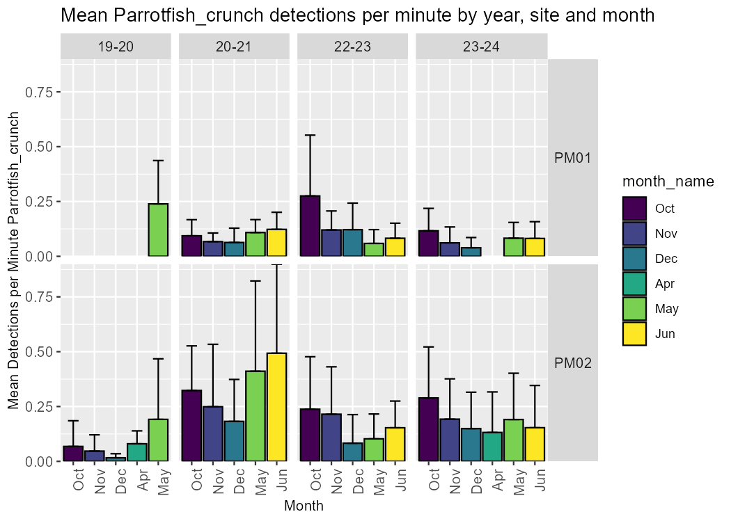
Parrotfish activity (crunching on the reef) was counted and averaged per minute each day across 700 daylight minutes (the hours when parrotfish are active on the reef) to estimate a monthly average of parrotfish activity. This figure shows the monthly means of parrotfish activity (crunch rate) at the PM01 and PM02 monitoring locations between 2019 and 2024. There was no data for 2021-22. Error bars represent the standard deviation across daily activity means within each month. Therefore, using the y-axis, monthly parrotfish activity can be understood as the mean per minute rate (e.g., 0.5) x 700 daylight minutes x number of days in a given month (e.g., 30). All data within peak humpback season (as defined in previous section) were removed, and months with fewer than 15 days of data were excluded. Credit: Conservation Metrics

We also present a metric of nighttime acoustic activity, calculated as the total number of fish calls detected during nighttime periods each night, aggregated across all sound classes. These nightly values were then averaged by month within each season. This metric is used as a proxy for nighttime reef soundscapes, capturing variability in biological acoustic signals during a period when many reef organisms are known to be active. It is motivated by studies showing that fish and coral larvae often settle at night, and that coral reef soundscapes can influence larval settlement.

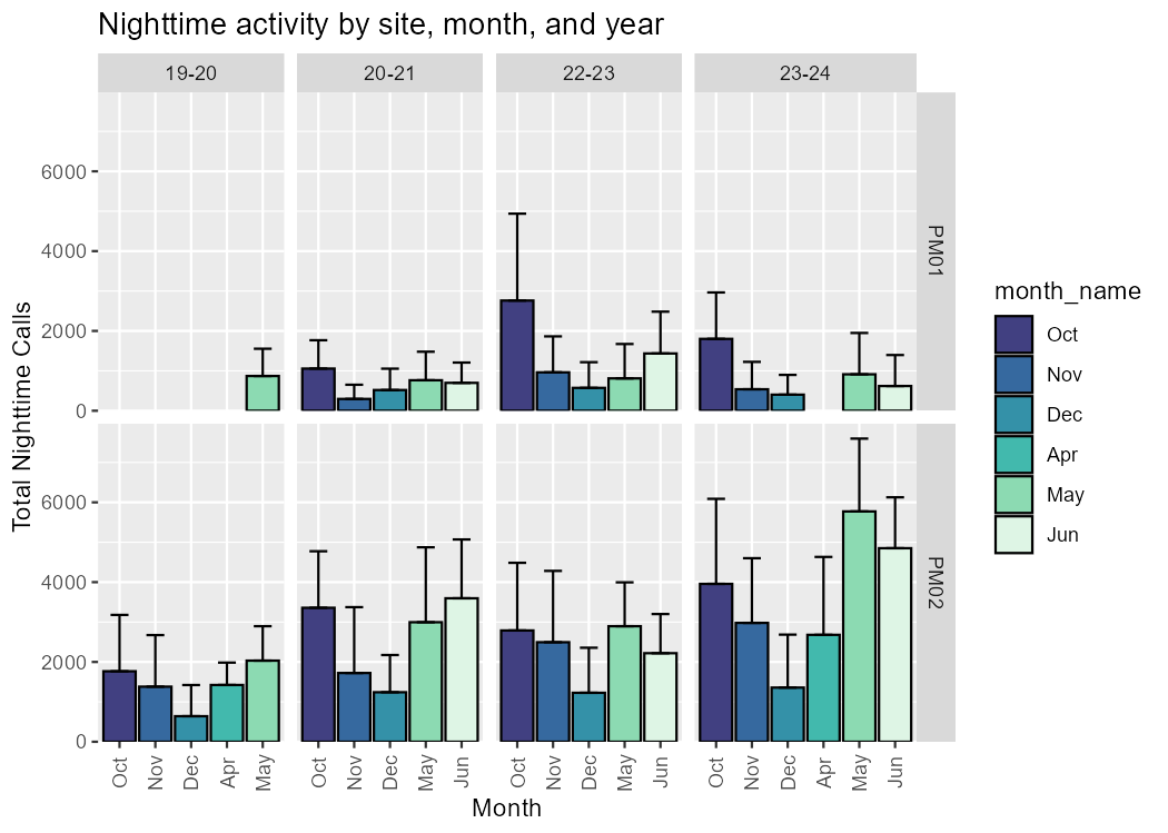
Nighttime fish activity (total fish calls detected during nighttime periods) was summed each night (30 minutes before sunset to 30 minutes after sunrise, based on local sunrise and sunset times). PM01 and PM02 were recorded on a 50% duty cycle. To ensure comparability across sites with different sampling regimes (including 50% duty cycle and continuous recording), nighttime detections were scaled to full-night equivalents based on recording effort. These nightly values were then averaged by month within each season to estimate monthly nighttime activity. This figure shows monthly means of nighttime fish activity at the PM01 and PM02 monitoring locations between 2019 and 2024. There was no data for 2021–22. Error bars represent the standard deviation across nightly activity values within each month. All data within peak humpback season (as defined in the previous section) were removed, and months with fewer than 15 nights of data were excluded. Credit: Conservation Metrics