Monterey Bay National Marine Sanctuary Soundscape Report

Ocean Sound Monitoring

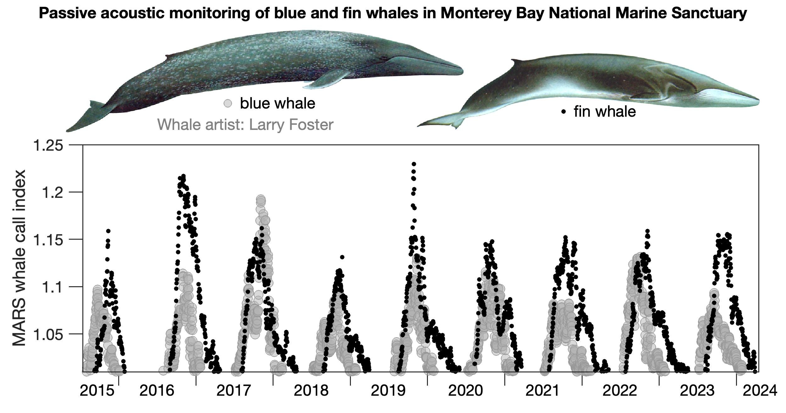
Ocean sound monitoring in Monterey Bay National Marine Sanctuary (MBNMS) coordinated by ONMS began in 2018 through the Sanctuary Soundscape Monitoring Project. This sanctuary has a long history of underwater acoustic monitoring dating back to measurements in the 1950s by the U.S. Navy near Point Sur Ridge. The Monterey Bay Aquarium Research Institute (MBARI) supports a continuous real-time monitoring effort within the sanctuary that began in 2015, known as the Soundscape Listening Room. Collectively, these underwater sound monitoring efforts have provided key insights on cryptic species, whale migration patterns and drivers, methods for detecting fish sounds, and steady rise in ocean noise levels, to highlight a few.

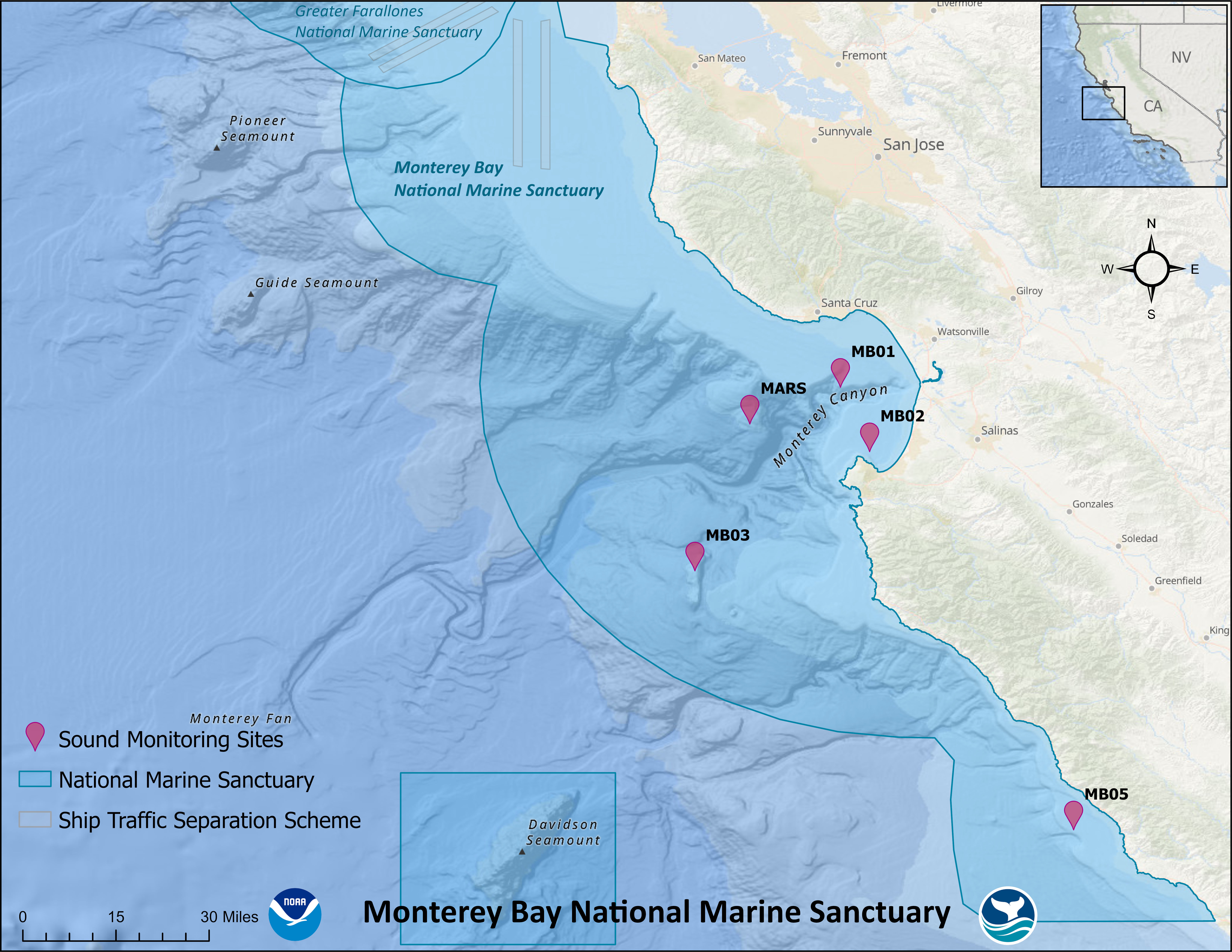
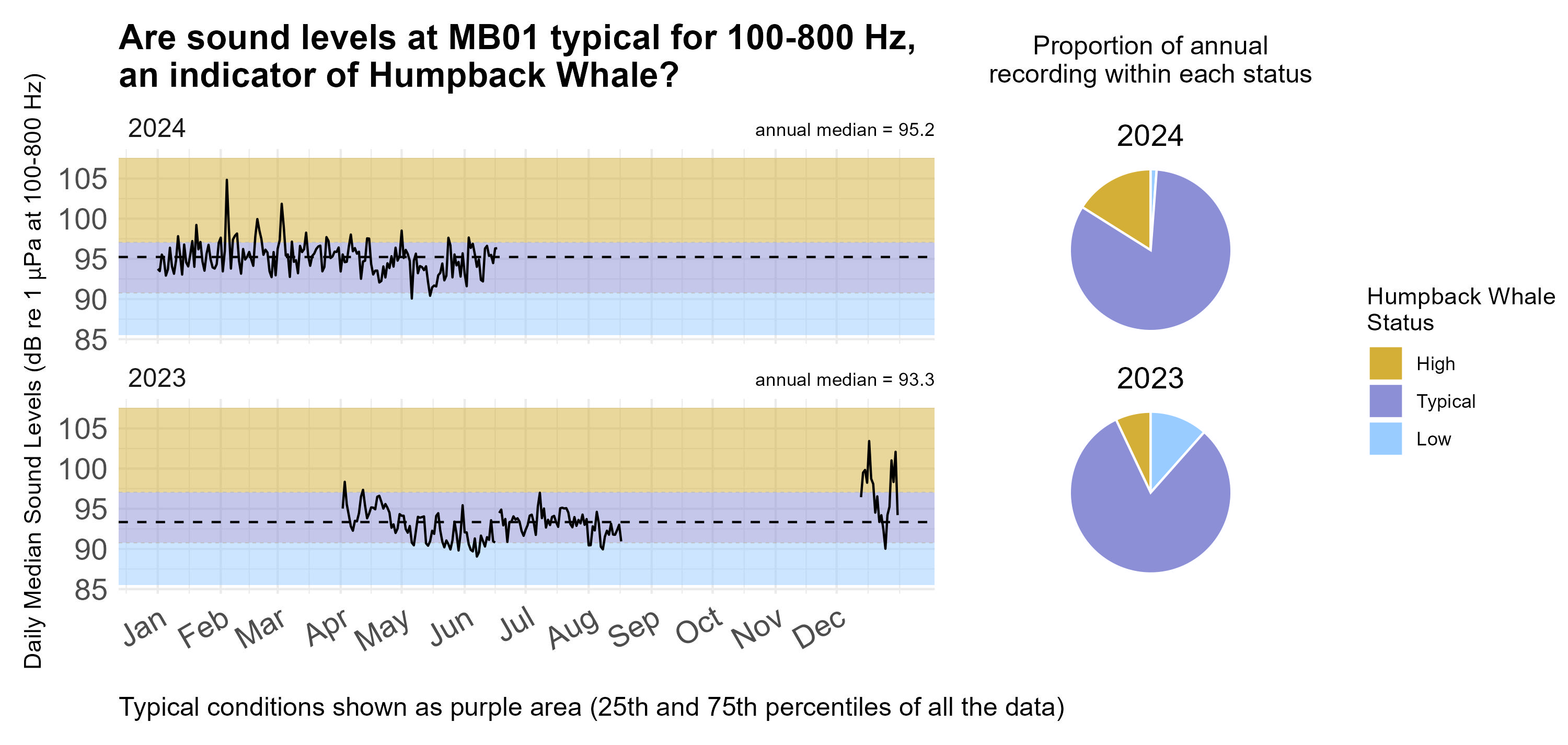
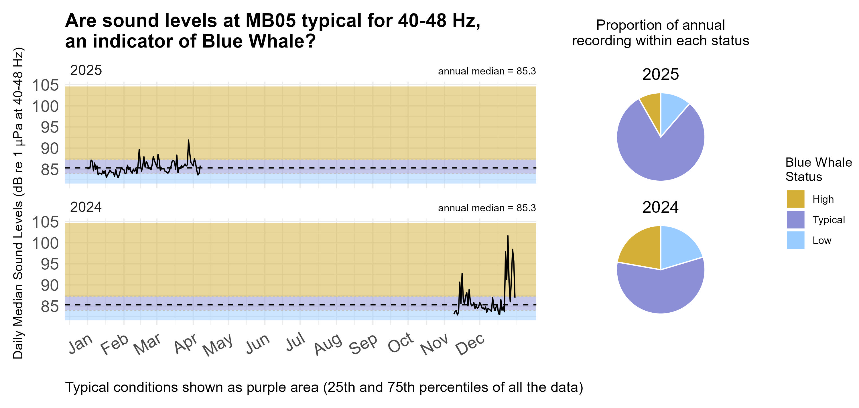
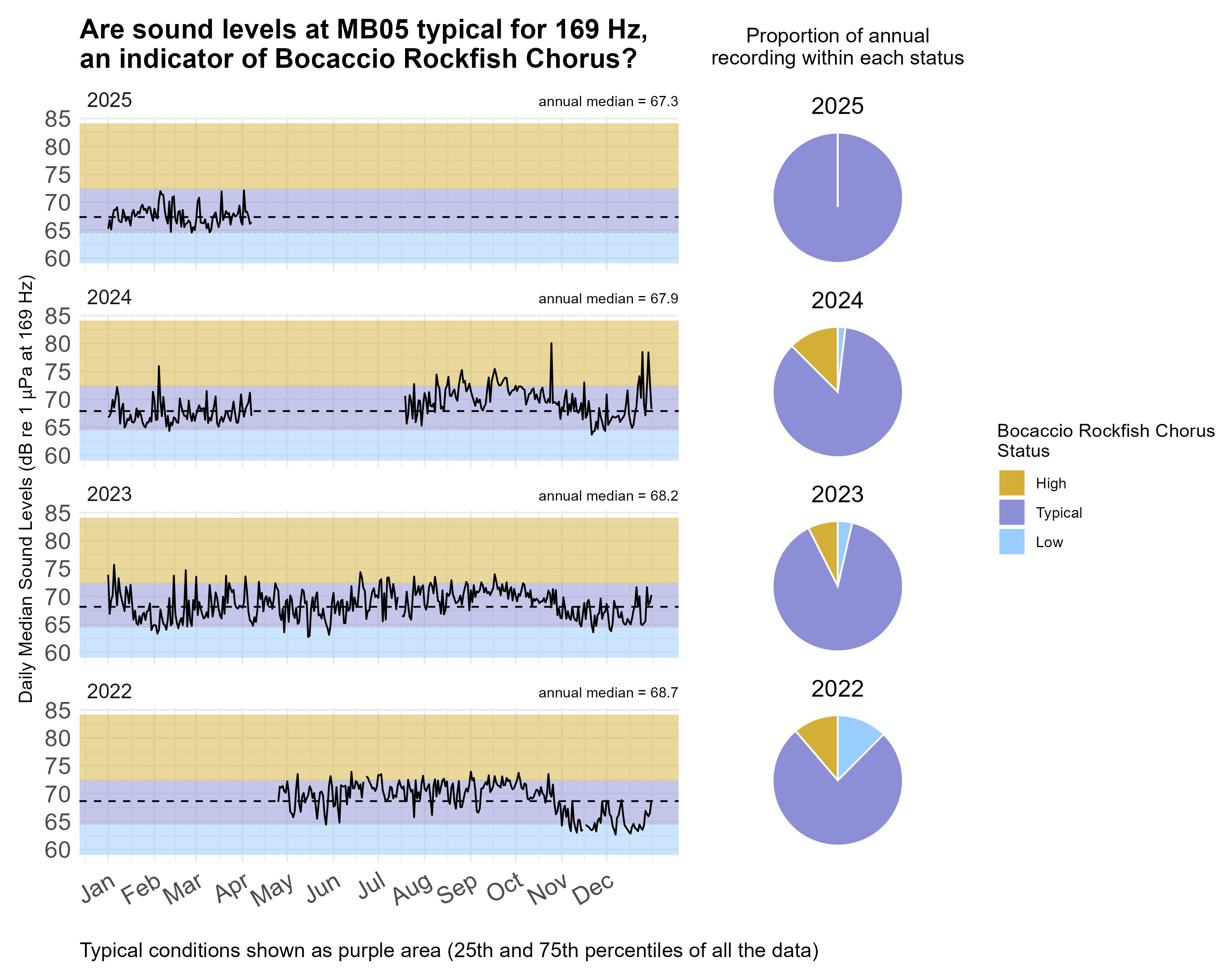
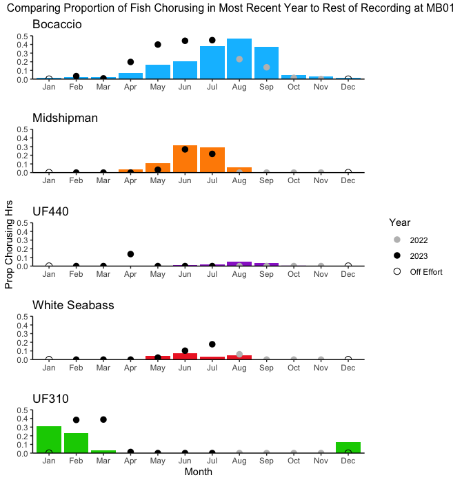
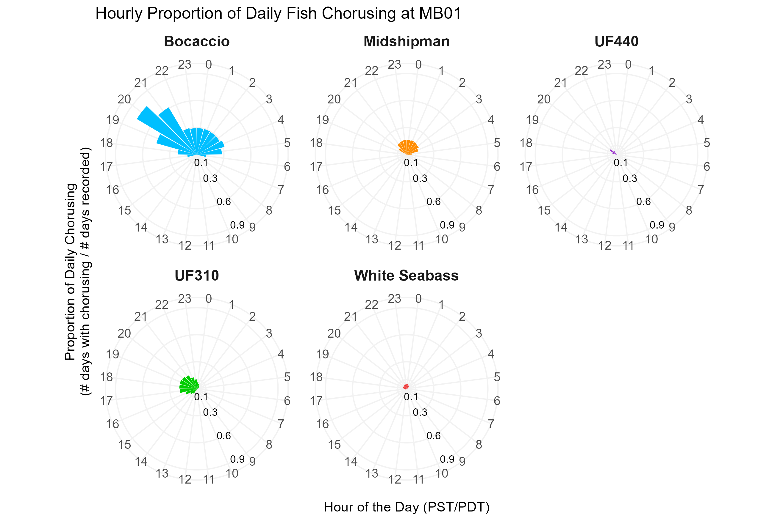
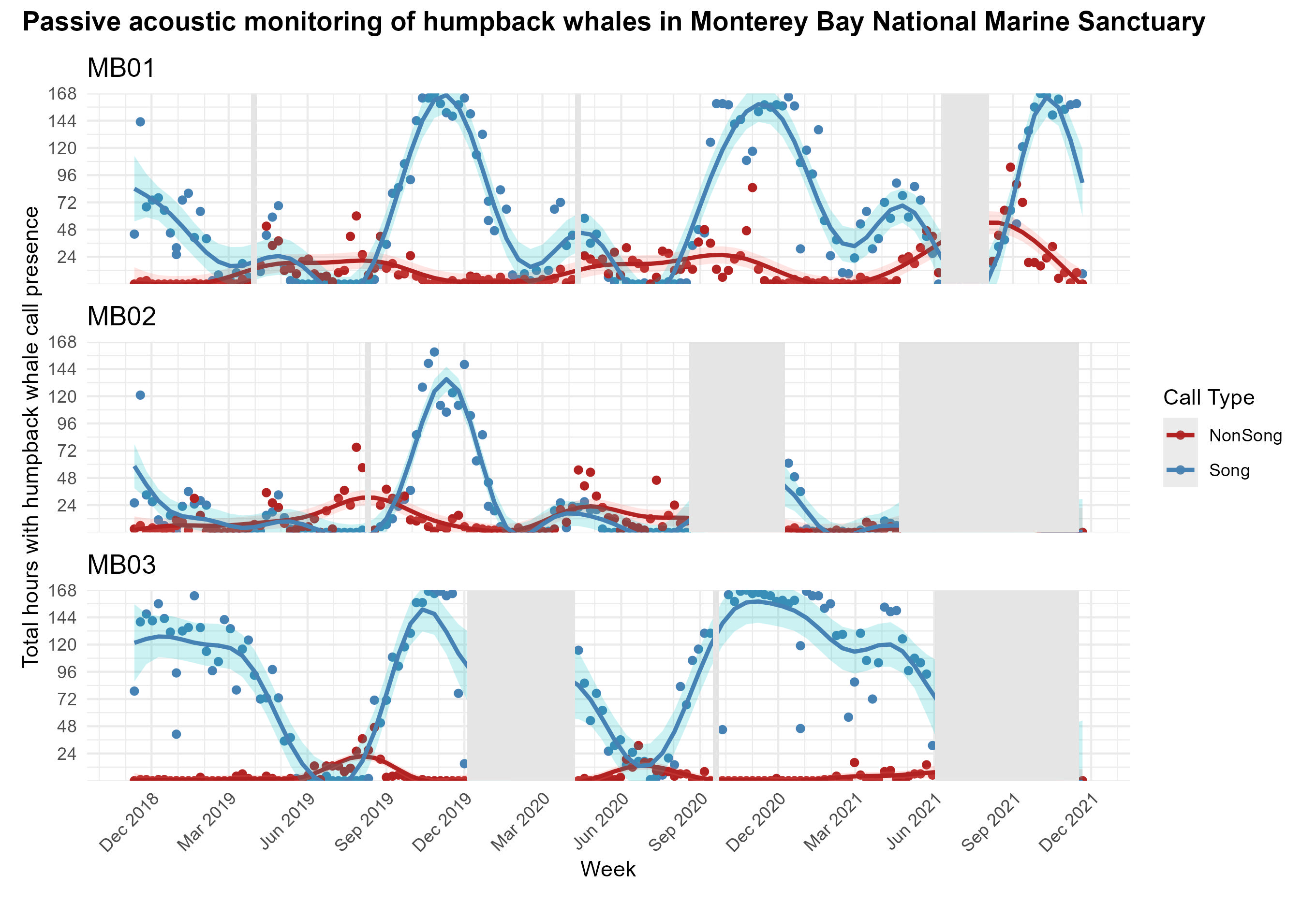
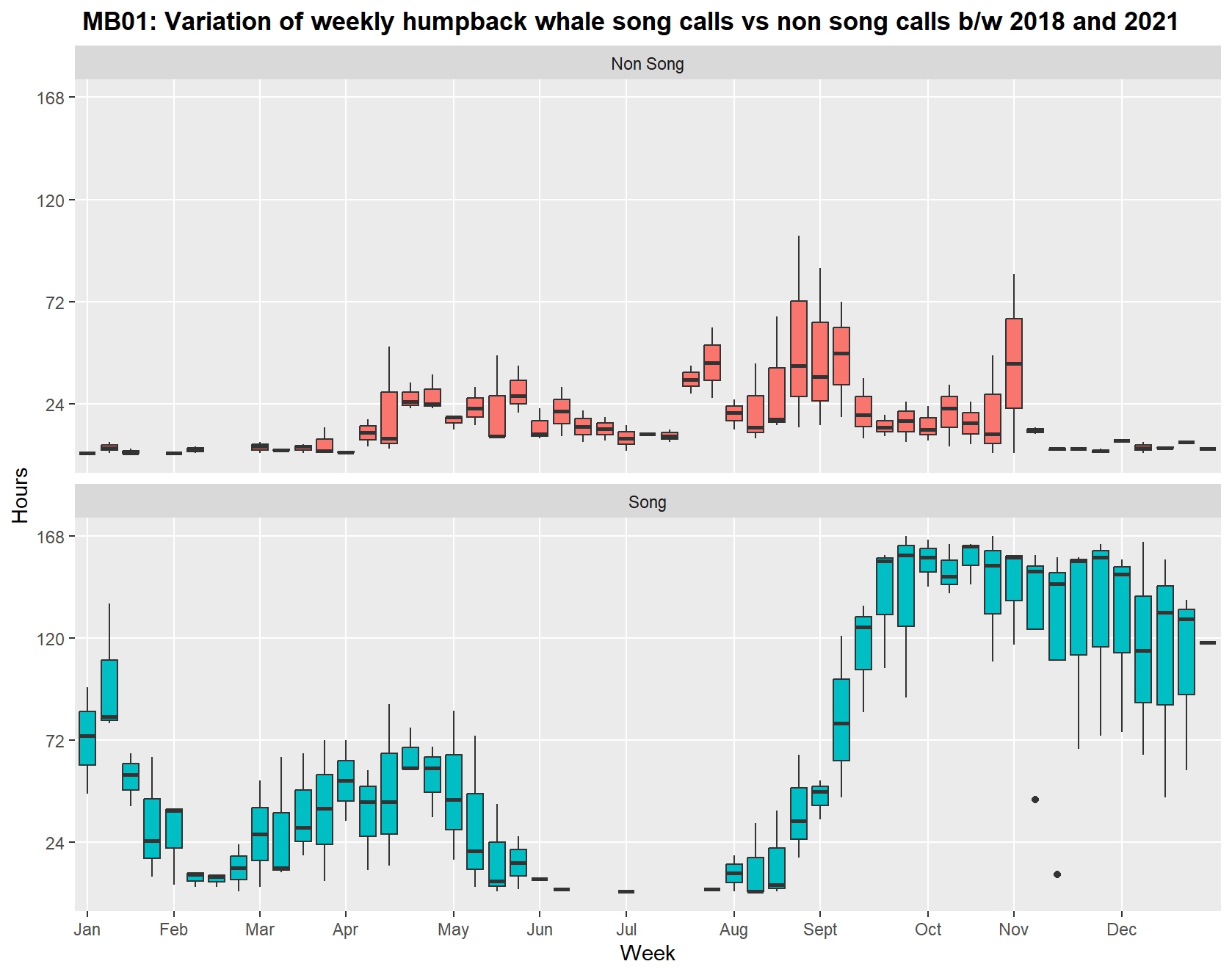
Current ONMS ocean sound monitoring and analysis is maintained at four locations in the sanctuary, as well the MBARI hydrophone. These four sites capture unique soundscapes. MB01 is in the middle of Monterey Bay, and on the edge of Monterey Canyon. That location is busy with foraging animals and vessels for commercial and recreational activities including fishing, whale watching and occasional visits from large cruise ships. MB02 is adjacent to four marine protected areas and is in rich kelp forest habitat; this shallow area off Point Pinos has a lot of vessel traffic in and out of Monterey Harbor. MB03 is offshore near transit lanes for ships weighing 300+ gross tons. This is a deep water area teeming with wide-ranging marine mammals, such as whales and dolphins. This site has decades of broadband sound data in its time-series and is managed by our partners at the Naval Postgraduate School. MB05 is located in La Cruz canyon, part of the understudied Big Sur coast, and recognized as an area of special ecological significance just inside the southern boundary of Monterey Bay NMS. This is the only California site where we hear bocaccio rockfish chorusing year round, and is an important MBARI blue whale observatory. This site is collaboratively maintained by sanctuaries and MBARI, and is adjacent to the Morro Bay wind energy development area.

To see historical monitoring sites that are no longer active, please visit Sanctuary Soundscape Project data portal.

Summary of monitoring sites

Long-term Monitoring Site	Primary Monitoring Purpose	Oceanographic Setting	Depth (m)	Sampling Rate (kHz)	Known Biological Sounds	Vessel Traffic Setting	Latitude	Longitude	Start Date	Total Recording Days
MB01	To monitor foraging whales, chorusing fish, and vessel noise.	coastal-shallow, near Monterey Bay submarine canyon	116	48	Seasonal patterns driven by upwelling, with known sounds from baleen whales, pinnipeds, dolphins, fish, and snapping shrimp	Frequent recreational activity: whale watching and fishing	36.8	-121.98	Feb 2023	326.0
MB02	To monitor vessel traffic in and out of Monterey Harbor, and the vibrant kelp forest community.	coastal-shallow, adjacent to kelp forest ecosystems	72	48	Seasonal patterns driven by upwelling, with known sounds from baleen whales, pinnipeds, fish, and snapping shrimp	Frequent recreational activity: whale watching and fishing	36.65	-121.91	June 2022	684.0
MB03	To continue long-history of monitoring trends in ocean noise, marine mammals, and large vessels; ocean sound monitoring began in 1950s.	coastal-deep, on contiential slope in a well-studied area called Sur Ridge	855	200	Seasonal patterns driven by upwelling, with known sounds from baleen whales and dolphins	In the middle of offshore transit lanes for commercial shipping traffic	36.37	-122.31	Nov 2018	nan
MB05	To monitor bocaccio rockfish chorusing and blue whale seasonality in La Cruz Canyon in MBNMS special ecological significance area (SESA) #15.	coastal-shallow, on the continental shelf in La Cruz Canyon off the Big Sur Coast	92	48	Seasonal patterns driven by upwelling, with known sound from baleen whales and fish. Tagged blue whales and leatherback sea turtles use this habitat. This is the only monitoring location with year round boccacio fish presense, suggesting that La Cruz Canyon may be an important habitat for the commercially fished species.	La Cruz canyon is part of the understudied Big Sur coast just inside the southern boundary of Monterey Bay NMS and adjacent to the Morro Bay wind energy development area. Establishing baseline understanding of biological presence and vessel traffic is important ahead of any increase in offshore development.	35.767783	-121.433433	Apr 2022	nan
MARS	Long-term monitoring of marine mammals and vessel noise, including real-time detection capability.	coastal-deep, on contiential shelf in the middle of Monterey Canyon on Smooth Ridge	890	256	Listen to the live feed!	Commercial ship traffic is consistent along the western edge of MBNMS, and numerous smaller commercial, fishing, and leisure boats transit within the sanctuary and are recorded at this site.	36.71	-122.19	July 2015	nan

Ocean Sound Conditions

Soundscapes vary across years, seasons, and even within a day. Differences are driven by shifts in wind and weather patterns, migration and behavior of animals, and patterns in human activities. We track how sound levels change in different frequencies using standardized soundscape metrics to understand these changes. Seasonal and annual percentiles of all the data, a measurement of data spread with the middle 50% falling between the 25th and 75th percentile, are used to define typical conditions.

What are the seasonal patterns across frequencies?

Season is often a main driver of soundscape differences: wind and weather patterns shift, species migrate or change behavior, and humans change their marine activities. As shown on the graphic(s) below, we can visualize the differences by looking at the variation across frequency (pitch of the sound in Hertz) shown on the x-axis and intensity (how loud the sound is in decibels) shown on the y-axis. The colored lines represent regionally-specific oceanographic seasons, vertical shaded bars are the frequency ranges that a sound source of interest can be heard, and the black lines bound the expected range of modeled sound intensity when only wind noise is present.
Here are some questions to consider when viewing the graph(s) below:
(1) Which season has the highest sound levels?
(2) Are there peaks in the sound levels for any of the sounds of interest?
(3) Are the low-frequency sound levels outside the expected range for wind noise?

Seasonal median sound levels (sound intensity measured by mean-square pressure in microPascal per Hertz) across a range of frequencies (~10 to ~24,000 hertz) at a given monitoring site, with annual recording effort represented by a bar graph underneath. Each season is a different colored line. Solid black lines show modeled ambient sound levels from wind at 1 m/s (lower line) and 22.6 m/s (upper line) based on hydrophone depth. Frequency bands indicative of a biological or anthropogenic sound source of interest are highlighted in semi-transparent gray and labeled; peak frequency for dominant fish species are labeled with vertical dashed lines. Credit: Megan McKenna and Emma Beretta/CIRES and NOAA

Processing raw audio files to calibrated sound levels (i.e., soundscape metrics) involves multiple steps to get a specified time frequency data product. All soundscape metrics visualized in the soundscape inventory reports are averaged from hybrid millidecade sound levels, calculated using either MANTA or PyPAM software packages. Both softwares calculate mean PSD (dB re 1 µPa^2/Hz) per minute in 1-Hz wide bins using Welch’s method with a Hann window, FFT length equal to the sample rate, and 50% overlap. Following calibration based upon instrument specific sensitivities, PSD values per minute were further processed in hybrid millidecade spectral densities, which are an efficient means of storing PSD spectra from high sample rate audio files using 1-Hz values up to 435 Hz, and then millidecade wide PSD values up to one half of the sample rate (Martin et al. 2021).

PAMscapes was used to calculate hourly median hybrid milli-decade bands (loadSoundscapeData(ncFile, keepQuals = c(1,2)) and binSoundscapeData(hmddata, bin = "1hour", method = c("median")). The hourly data were then matched with an estimate of wind speed at that location using matchGFS in PAMscapes (Global Forecast System (GFS) weather model). Long-term condition plots in these reports were generated by averaging the hourly median hybrid millidecade results within different time constraints (i.e. annual, seasonal) and percentiles (e.g., 25% and 75%) for each hybrid millidecade frequency band.

How are ocean sound conditions changing across years?

We can track changes in ocean soundscape conditions and its contributors by comparing annual sound levels. Efforts to reduce noise impacts to marine animals are underway on local to global scales. Strategies can include avoidance of times and areas when sensitive species are present to reduce vulnerability (e.g., a shipping lane), changing the operation of a potentially hazardous noise source (e.g., by slowing and therefore quieting vessels) or through the design and use of alternative, quieter sources (e.g., new, quieter ship design and/or technologies). The effectiveness of these approaches, and the scales over which they are effective, can be tracked through comprehensive monitoring efforts. A focused analysis is often necessary to tease apart the multiple drivers of ocean sound levels, however, annual summaries provide initial insights to overall patterns.
Here are some questions to consider when viewing the graph(s) below:
(1) Are levels lower in the most recent year of monitoring in any of the frequencies of interest?
(2) Are there peaks in the sound levels for any of the sounds of interest? Do they differ across years?

Annual median sound levels (sound intensity measured by mean-square pressure in microPascal per Hertz) across a range of frequencies (~10 to ~24,000 hertz) at a given monitoring site, with annual recording effort represented by a bar graph underneath. Each year is a different blue line, getting darker for every additional year of data. Solid black lines show modeled ambient sound levels from wind at 1 m/s (lower line) and 22.6 m/s (upper line) based on hydrophone depth. Frequency bands indicative of a biological or anthropogenic sound source of interest are highlighted in semi-transparent gray and labeled; peak frequency for dominant fish species are labeled with vertical dashed lines. Credit: Megan McKenna and Emma Beretta/CIRES and NOAA

Is the intensity (loudness) of sound sources of interest within typical range?

In some soundscapes, we can use specific frequencies as indicators for the presence of a source of interest (e.g. species presence and behavior). Monitoring sites are often chosen because a known source that we want to track is present and we can track this dominant sound energy contributor using their specific frequency or frequency range. For example, seasonal migration of humpback whales to Hawaiian Islands results in soundscapes dominated by their calling between 50 and 630 Hz. At sites near commercial shipping lanes, 63 and 125 Hz one-third octave level (TOL) are used as an indicator for ship noise (Haver et al. 2021)). At sites where snapping shrimp are present, 4,000 - 18,000 Hz can be used as an indicator of their sounds. Only frequencies that have been identified as reliable for tracking a source of interest are shown below.

Time series plot of daily median sound levels (sound intensity measured by mean-square pressure in microPascal per Hertz) for a specific frequency band(s) of interest at this site, separated by year. Background color shading (blue, purple, gold) indicates low (<25th percentile), typical (25-75th percentile), and high sound levels (>75th percentile) across this monitoring site's entire dataset at this frequency band(s) for comparability with annual medians, marked with horizontal black dashed lines. Pie charts on the right hand side of the graphic show the proportion of daily median sound levels that fell within each category for each year, following the same color-coding and percentile bins. Credit: Megan McKenna and Emma Beretta/CIRES and NOAA

Ocean Sound Indicators

We can use long-term monitoring of ocean sound to derive and track indicators of ocean conditions. These indicators track the status and trend of habitat condition, species presence, human-use patterns, and management activities. There are many analytical methods used to generate ocean sound indicators. Below are ocean sound indicators relevant to the sanctuary and available for condition tracking.

When does fish chorusing contribute to the soundscape?

Knowing when fish are calling helps identify important biological periods for fish species. A reduction in noise during these periods benefits fish communication. Use the graphics below to identify months of the year and times of the day with higher levels of fish chorus. For a more details on the analysis check out: Spatiotemporal patterns of fish chorusing in California National Marine Sanctuaries.

Bar plot indicating the proportion of time that chorusing was detected each month based on the 3-year period from January 2019 to December 2021, for bocaccio (Sebastes paucispinis), plainfin midshipman (Porichthys notatus), white seabass (Atractoscion nobilis), and two unknown fish species UF440 and UF310 at listening station MB01 in Monterey Bay National Marine Sanctuary. Dots show the proportion of chorusing hours for the most recent recording year, which was from August 2022 to July 2023. Grey dots are for 2022, black dots for 2023, and empty dots for off effort (no data those months). Credit: Emma Beretta/CIRES and NOAA

Radial plots showing the proportion of sampled acoustic data containing detections of fish chorusing, summarized by hour of day, for bocaccio (Sebastes paucispinis), plainfin midshipman (Porichthys notatus), white seabass (Atractoscion nobilis), and two unknown fish species UF440 and UF310 at listening stations MB01, MB02, and MB05 in Monterey Bay National Marine Sanctuary. Recording at MB01 spanned from November 2018 to August 2023, MB02 recording spanned from November 2018 to July 2023, and MB05 recording spanned from April 2022 to July 2023. Daily chorusing activity for each fish species is the number of days with chorusing presence per number of days recorded. Credit: Emma Beretta/CIRES and NOAA

When are the seasonal biologically-important times for whales?

MBNMS represents important foraging habitat for multiple whale species. In the heart of MBNMS, the MARS cabled observatory enables continuous monitoring of sound. Scientists at the Monterey Bay Aquarium Research Institute (MBARI) track the acoustic presence of whale species in this region. Beyond indicating presence, acoustic monitoring enables research into whale behavioral ecology, which is essential to inform conservation. In addition to the seasonal detection of mysticete species like blue and fin whales (below), continuous listening reveals that the largest odontocete species – the sperm whale – is present year-round even though it is rarely seen.

The occurrence of blue (Balaenoptera musculus) and fin (Balaenoptera physalus) whale song detected by Monterey Bay Aquarium Research Institute’s MARS underwater cabled listening station in Monterey Bay since 2015. The y-axis indicates whale call index (Oestreich et al., 2020) which is a metric of blue and fin whale B call intensity, rather than individual call detection. Credit: John Ryan/MBARI

The Office of National Marine Sanctuaries (ONMS) maintains three MBNMS listening stations with the Naval Postgraduate School, MB01, MB02, and MB03. We partnered with Moss Landing Marine Laboratories and Stanford Hopkins Marine Station to analyze data from these three sites for humpback whale vocalization, both song and non-song calls, to understand seasonality and potential behavior associated with calls over time. For a more details on the analysis check out: Acoustic Presence of Humpback Whales in U.S. West Coast National Marine Sanctuaries

The total number of humpback whale (Megaptera novaeangliae) song (blue dots) or non-song vocalizations (red dots) detected during a given week from November 2018 to December 2021 at three listening stations MB01, MB02, and MB03 in Monterey Bay National Marine Sanctuary. Shaded grey regions indicate weeks with reduced recording effort (less than 75% of the week, or <126 recording hours). The smoothed blue curve highlights seasonal patterns in whale calling activity, modeled using a generalized additive model (GAM), and the shaded band surrounding it represents the model-estimated 95% confidence interval. Credit: Emma Beretta/CIRES and NOAA

Boxplots showing weekly variability in total number of hours of detected humpback whale vocalizations aggregated across years from 2018 and 2021, comparing non song and song call types. Credit: Generated using PAMscapes version 0.15.0 (Sakai et al., 2025)